Getting Started
This quickstart guide will help you train a pRNN model. We’ve implemented tutorial.ipynb in the package repo, so that you may run the preliminary analysis yourself. When using this package, you’ll be primarily working with three objects.
An environment object, defined in
env.py. Along with theShellobject, it serves as the interface between external environment packages (e.g.gym,minigrid,RatinaBox) and any models defined by our packages. These objects contain getter/setter methods, along with tools to convert inputs into datatypes suitable for the pRNN.An agent object, defined in
agent.py. This defines how actions are taken within the environment and maintains astateattribute that keepts track of the agent’s position and head direction over time.A
predictiveNetobject. This is the object that contains the network. This network learns to predict egocentric sensory observations as the agent moves around the environment. As a result, the predictveNet develops a cognitive map of the environment. It contains utilities to manage training steps of the network, such as producing predictions and adjusting weights, as well as plotting functionality.
For this quickstart tutorial, you’ll want to install the minigrid package from Farama Foundation into your environment. You can do this by cloning the latest version onto your machine and pip installing it in editable mode:
git clone git@github.com:Farama-Foundation/Minigrid.git
pip install -e .
Make sure to also install the pRNN package in editable mode as well. See the README for instructions on how to do this.
We’ll first import the predictiveNet class, which contains the machinery to train a pRNN model. We also import make_env and RandomActionAgent from utils. Environments are made to manage different scenarios in which pRNNs are trained in, varying by world environment package (e.g. gym-minigrid, farama-minigrid, Rat-in-a-Box, miniworld, etc), encoding of actions, and observation type. The RandomActionAgent will return a sequence of random actions for the egocentric agent to use while navigating the environment specified with make_env.
#import the pRNN class
from prnn.utils.predictiveNet import PredictiveNet

from prnn.utils.env import make_env
from prnn.utils.agent import RandomActionAgent

import matplotlib.pyplot as plt
import numpy as np
wandb not installed, will not log to wandb
Here, we specify which package will generate the world environment (here farama-minigrid), and in which particular setting the agent will be placed in (here LRoom-20x20-v0). For this particular run, we’ll also specify the encoding scheme for the actions. Head direction (forward, left, right, backwards) is one-hot encoded, and we also store agent speed. (#TODO confirm size).
#Make a gridworld environment
env_package = 'farama-minigrid'
env_key = 'LRoom-20x20-v0'
act_enc = 'SpeedHD' #actions will be encoded as speed and one hot-encoded head direction

env = make_env(env_key=env_key, package=env_package, act_enc=act_enc)
We specify the agent parameters:
#specify an action policy (agent)
action_probability = np.array([0.15,0.15,0.6,0.1,0,0,0])
agent = RandomActionAgent(env.action_space, action_probability)
Next, we construct the pRNN model. Note that the predictiveNet class recieves both the env variable as well as the type of pRNN we’re training. See the “Models” page for an explanation of which models are supported, as well as Architectures.py for a full list. Generally, we focus on three types: next-step prediction models, masked prediction models, and rollout models. Here, we choose to construct a pRNN with five timestep observations masked. If we set pRNNtype = "Masked", we may also like to provide additional keyword arguments to further specify the model; such as inMask_length, which sets the number of future observations that are masked, and useLN which determines whether or not to apply LayerNorm.
#Make a pRNN
num_neurons = 500
pRNNtype = "Masked"
predictiveNet = PredictiveNet(env, hidden_size=num_neurons, pRNNtype=pRNNtype, k = 5, use_LN = True)
Once the environment, agent, and network have been defined, it’s possible to plot a sample trajectory to provide an example of actions and observations. The following lines will plot the agent in the environment, show it’s egocentric view, and what it’s prediction is for that timestep. Note that the pRNN has not been trained yet, so predictions will be noisy dependent on the initialization scheme. By default, weights are initialzied uniformly according to the Xavier initialization scheme.
#run a sample trajectory (note: predictions will be garbage, agent is untrained)
predictiveNet.plotSampleTrajectory(env,agent)
plt.show()
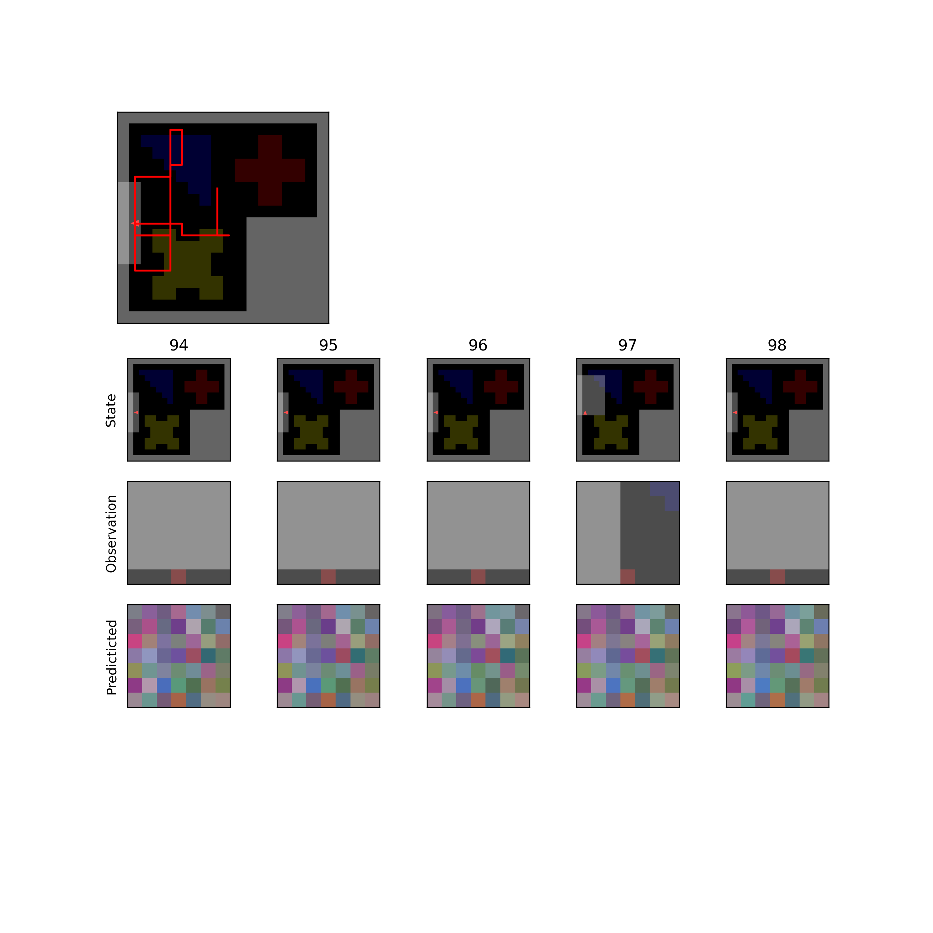
The agent’s predictions are all noise.
We can finally begin to train the network, after specifying some hyperparameters. Here, we set both hyperparameters to 50 for the sake of a quick(er) example run. We aren’t expecting any major performance increases with this. These two hyperparameters should ideally be set upwards of 500. That step may take a while!
#Run one training epoch of 500 trials, each 500 steps long
sequence_duration = 50
num_trials = 50

predictiveNet.trainingEpoch(env, agent,
                        sequence_duration=sequence_duration,
                        num_trials=num_trials)
Training pRNN on cpu...
loss: 0.028, sparsity: 3.9, meanrate: 0.38 [    0\   50]
loss: 0.022, sparsity: 3.9, meanrate: 0.39 [    5\   50]
loss: 0.02, sparsity: 3.9, meanrate: 0.39 [   10\   50]
loss: 0.016, sparsity: 3.9, meanrate: 0.39 [   15\   50]
loss: 0.019, sparsity: 4.0, meanrate: 0.39 [   20\   50]
loss: 0.017, sparsity: 4.0, meanrate: 0.39 [   25\   50]
loss: 0.018, sparsity: 3.9, meanrate: 0.39 [   30\   50]
loss: 0.016, sparsity: 4.0, meanrate: 0.39 [   35\   50]
loss: 0.017, sparsity: 4.0, meanrate: 0.4 [   40\   50]
loss: 0.015, sparsity: 4.0, meanrate: 0.4 [   45\   50]
loss: 0.016, sparsity: 4.0, meanrate: 0.39 [   49\   50]
Epoch Complete. Back to the cpu
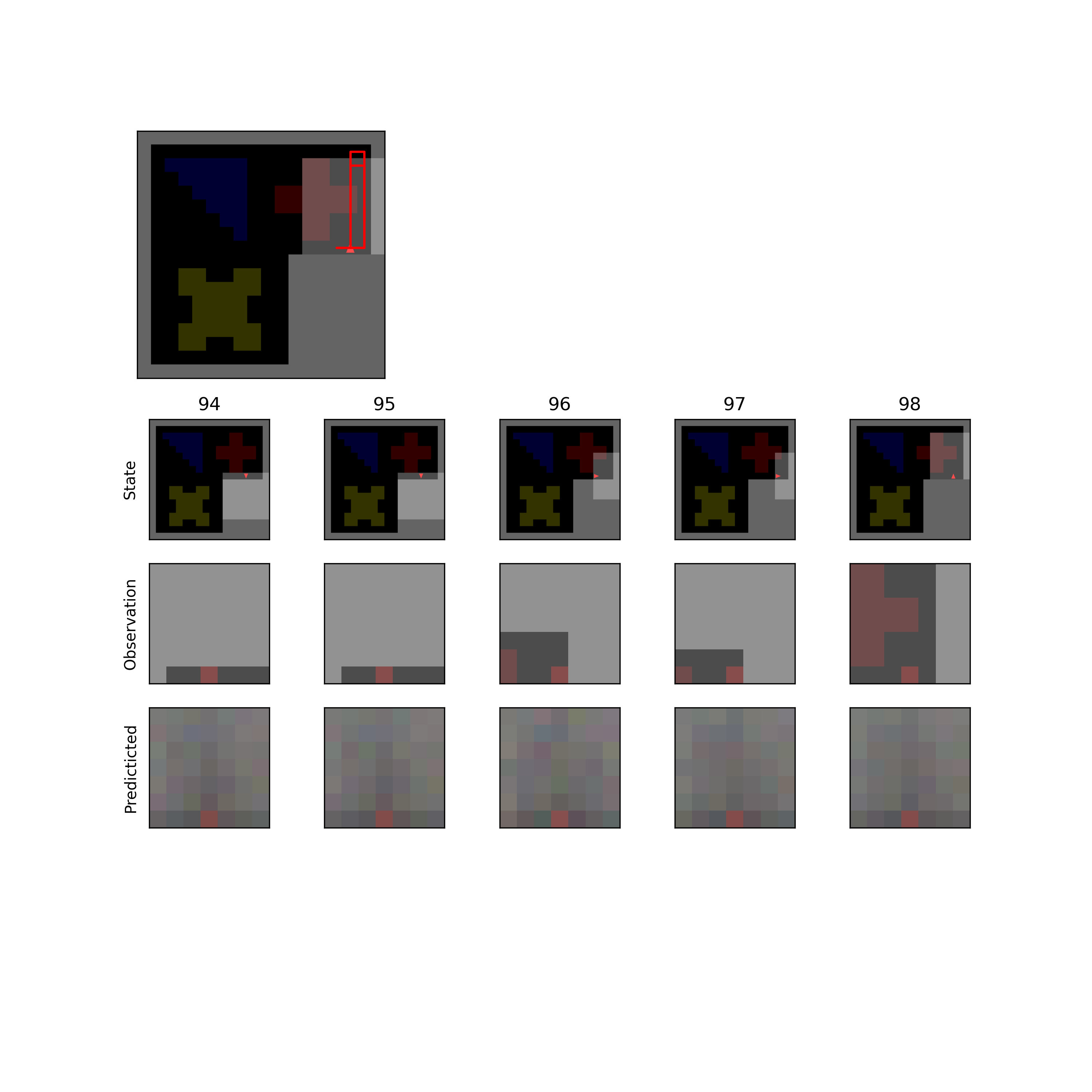
After the network trains, we can plot another sample trajectory to compare true and predicted observations. Did they get better? Training for more epochs should improve this performance. We can also inspect how spatial position is decoded, along with a panel of tuning curves.
#run a sample trajectory. did the predictions get better?
predictiveNet.plotSampleTrajectory(env,agent)
plt.show()

#Let's take a look at the spatial position decoding and tuning curves
place_fields, SI, decoder = predictiveNet.calculateSpatialRepresentation(env,agent,
                                                trainDecoder=True, saveTrainingData=True)

predictiveNet.calculateDecodingPerformance(env,agent,decoder)
predictiveNet.plotTuningCurvePanel()
Training Decoder on cpu...
loss: 5.870765 [    0\ 5000]
loss: 4.540343 [  500\ 5000]
loss: 4.259828 [ 1000\ 5000]
loss: 4.078527 [ 1500\ 5000]
loss: 3.957789 [ 2000\ 5000]
loss: 3.872919 [ 2500\ 5000]
loss: 3.810321 [ 3000\ 5000]
loss: 3.761265 [ 3500\ 5000]
loss: 3.684167 [ 4000\ 5000]
loss: 3.669147 [ 4500\ 5000]
loss: 3.618855 [ 4999\ 5000]
Training Complete. Back to the cpu
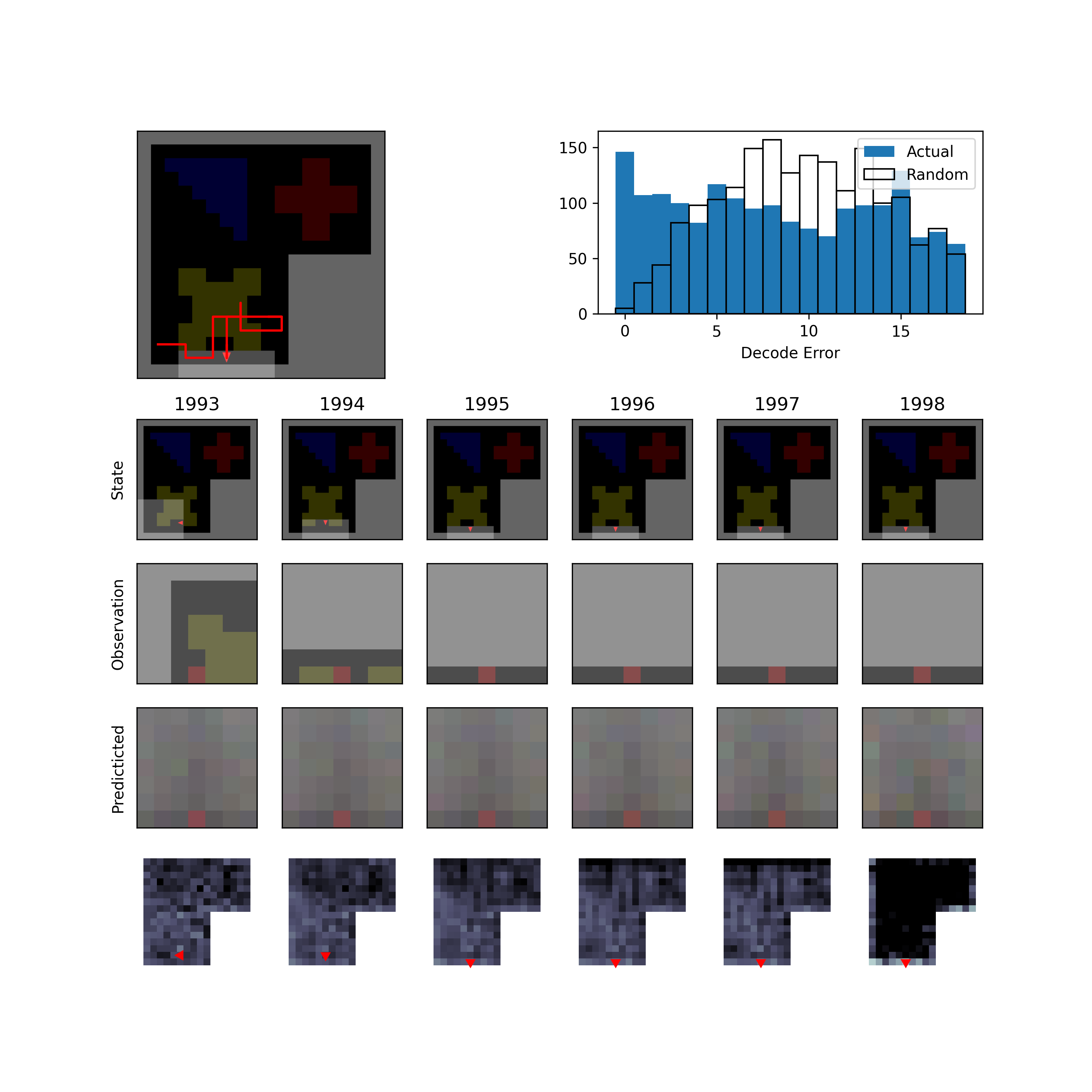
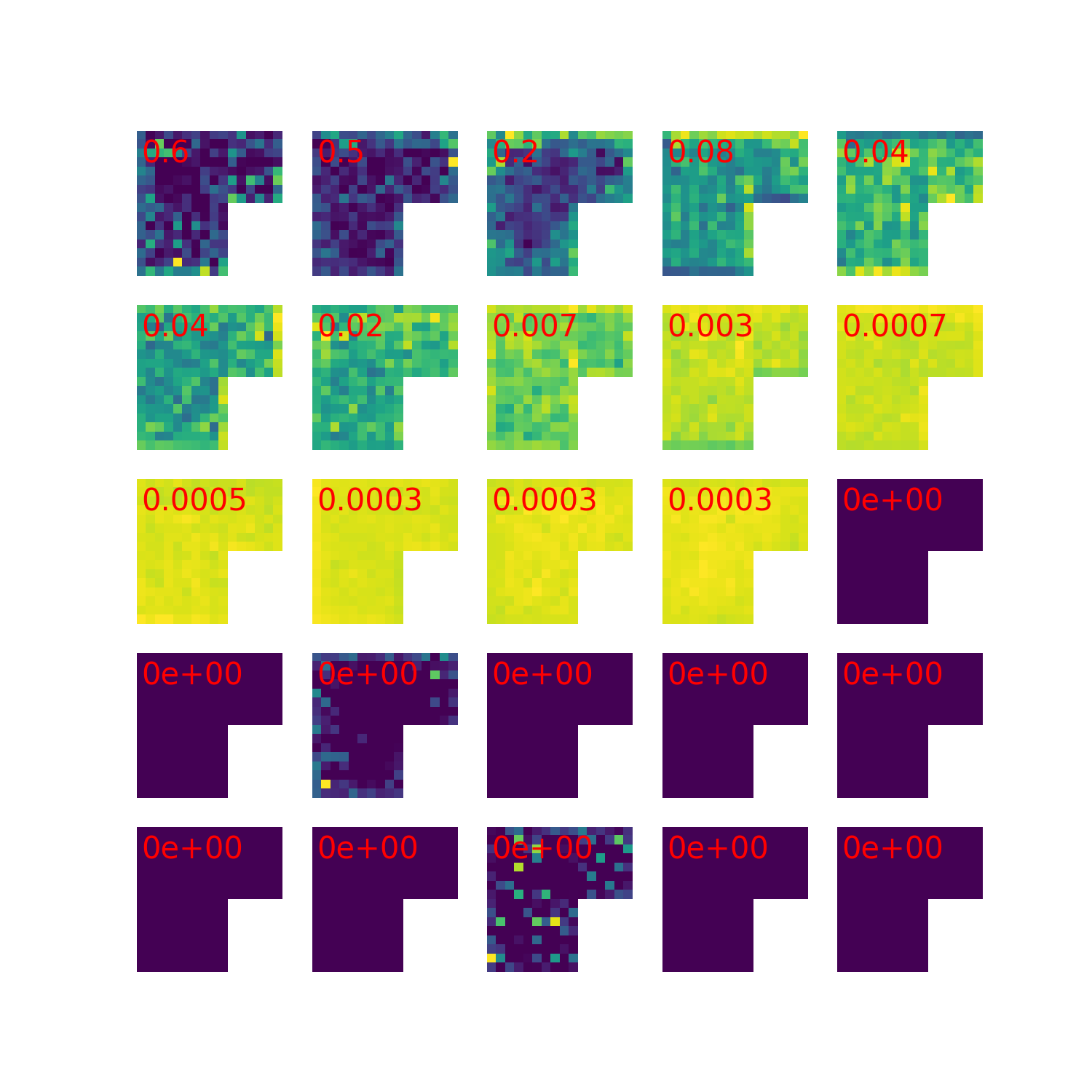
The agent’s predictions are still noisy, but we can see the predictions more informed by the egocentric perspective. Note that calculateSpatialRepresentation calls collectObservationSequence which generates a sequence of agents observations and actions and predict which does the forward pass (generating an predicted observation and updated hidden state). It’s important to understand how the shape of the model’s state changes given the type of network used. Running the below will be informative. Here, we collect 10 timesteps of information, then do a forward pass.
obs, act, state, render = predictiveNet.collectObservationSequence(env,agent,10,discretize=True)
obs_pred, obs_next, h  = predictiveNet.predict(obs,act, fullRNNstate=False)
print(h.shape)
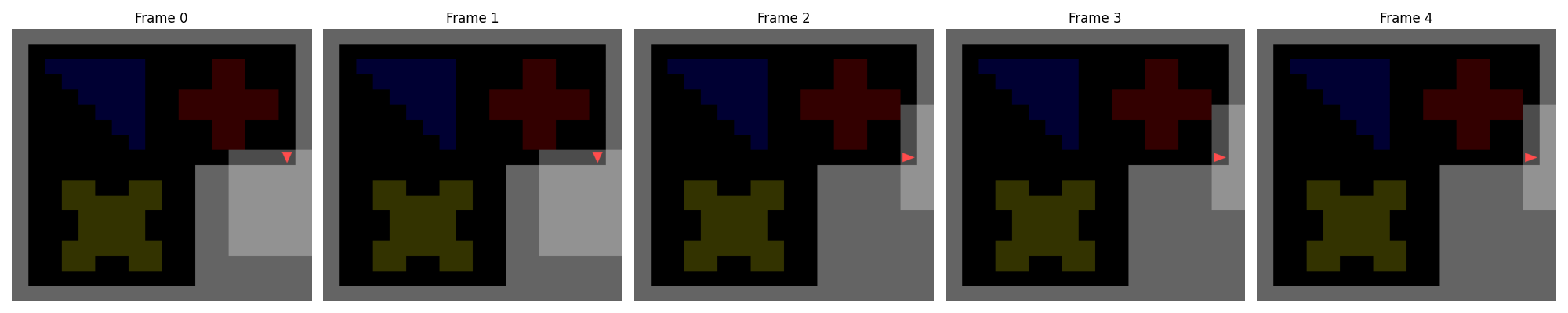
The shape of the hidden state, h, depends on whether the model batches, and on whether rollouts are performed. For the prnn.utils.Architectures.NextStepRNN and prnn.utils.Architectures.MaskedRNN, the shape of h will be [1, T, N] where T is the number of timesteps, and N is the number of neurons in the network. If we train with batching (call this B), an extra dimension gets added to the end [1, T, N, B]. In the case of prnn.utils.Architectures.RolloutRNN, the shape of h will be [k, T, N, B] where k is the number of rollout steps. Note that state is not the same as h. The state variable is a dictionary that holds a record of the agents positions and head direction over time. The render either remains set as False, or contains a list of rendered frames for display. For example:
fig, axes = plt.subplots(1, 5, figsize=(20,4))

for i, ax in enumerate(axes):
    im = ax.imshow(render[i], aspect = 'auto')
    ax.set_title(f"Frame {i}")
    ax.axis('off')

plt.tight_layout()
plt.show()
After training, you will likely want to save the network for later analysis. This can be done with the included predictiveNet.saveNet() method, which accepts arguments to specify save name and location. Essentially, this method serializes (“pickles”) the network for later use, and handles other object attributes that cannot be serialized.
predictiveNet.saveNet(savename="Masked_k5", savefolder="nets/")
Note that there is also a corresponding predictiveNet.loadNet() that unpickles the network, restores any needed attributes, and performs additional configuration.
You can check out the models page to learn more about which types of models are suppored with predictiveNet, or the prnn.utils.Architectures documentation to learn how to build your own.
From the results above, it looks like we’d need to train some more. Often we like to precompute a dataset of random trajectories to speed things up. Check out the dataloader example for information on how to do this.
The script trainNet.py can be used to train a network for many epochs and save the results. This can be called in a bash scipt to submit a job using e.g.
python trainNet.py --savefolder='examplenet/' --lr=2e-3 --numepochs=6 --batchsize=16 --pRNNtype='Masked' --actenc='SpeedHD' --inMaskLength = 5 --useLN = True
You’ll want to modify it or make your own, to fit the needs of your own project. See the training and loading pRNNs page for more information on how to use this script.